5. Deep dive into leveraging real-time and forecasted data for flexibility
Recap of previous lessons
In the first two lessons, we introduced the concept of Sustainable IT Monitoring, some basics of the electricity grids, and relevant grid signals. We also discussed key considerations when selecting them and challenges associated with sourcing them. In the third lesson, we introduced the Sustainable IT Monitoring journey and conducted a deep dive on the first two steps of the journey in the last lesson: measuring IT emissions with higher granularity and adding further insights leveraging more grid signals.
Access last week’s lesson here for more details on the first two steps of a Sustainable IT Monitoring journey. Today, we will conduct a deep dive into the next and last two steps of the journey: leveraging real-time data and implementing automated load-shifting.
Next week, the last lesson will wrap up the course with a summary of the different topics addressed and the key takeaways.
Once again, we value all feedback received so far and encourage you to keep submitting your opinion on this course and the different lessons.
Please also submit any questions you may have so that we can address them as part of the final lesson next week. This week's feedback form also includes a field where you can ask questions for our QA section next week: 1 minute survey
In Today’s lesson, we'll look at optimizing our IT loads using various dimensions and signals.
Start optimizing your consumption with real-time data
The Sustainable IT Monitoring journey naturally starts with historical reports and dashboards presenting end-of-month statistics. This is already very valuable information for companies with a large IT footprint, or that service other companies. Data centers can build reports for their customers, for example, or a large enterprise can map its own IT infrastructure, and where and when their emissions come from.
If these represent a first step in the journey, enabling a better understanding of the current situation and identifying where opportunities lie as well as where management is most needed, moving closer to real-time represents a necessary third step in this maturity journey.
As highlighted during the previous lessons of this course, the state of the grid is very dynamic; it changes in space and time. This means that while historical data can be very useful for deriving best practices, such as favoring IT loads in the middle of the day in California and IT loads in the middle of the night in Ontario, moving to real-time data is a step needed to leverage the emissions and cost reduction potential of IT workloads.
Spatial flexibility
In the examples below, we go through Spatial load-shifting. Not every company will be able to do this, but two big categories can:
1. Companies that have a lot of cloud compute, hyperscalers, and data centers themselves, as well as their customers with large cloud infrastructures
2. Multi-location enterprises that have distributed owned IT infrastructure. Industries like Telecom, Banking, Pharma, and sometimes even heavy industry and manufacturing.
Optimising for emissions
Let’s take the example of us needing to run a workload on a data center. In this example, we have the choice between two data centers, one located in Ontario and one located in California. With historical data only, we would choose to run our workloads in Ontario, where the grid carbon intensity in August (134 gCO2/kWh) was almost half the one in California (242 gCO2/kWh). However, using real-time data would lead to more informed decisions. The cleanest grid actually depends on the time of the day since the two grids have completely different carbon intensity variations, as can be seen in the image below:
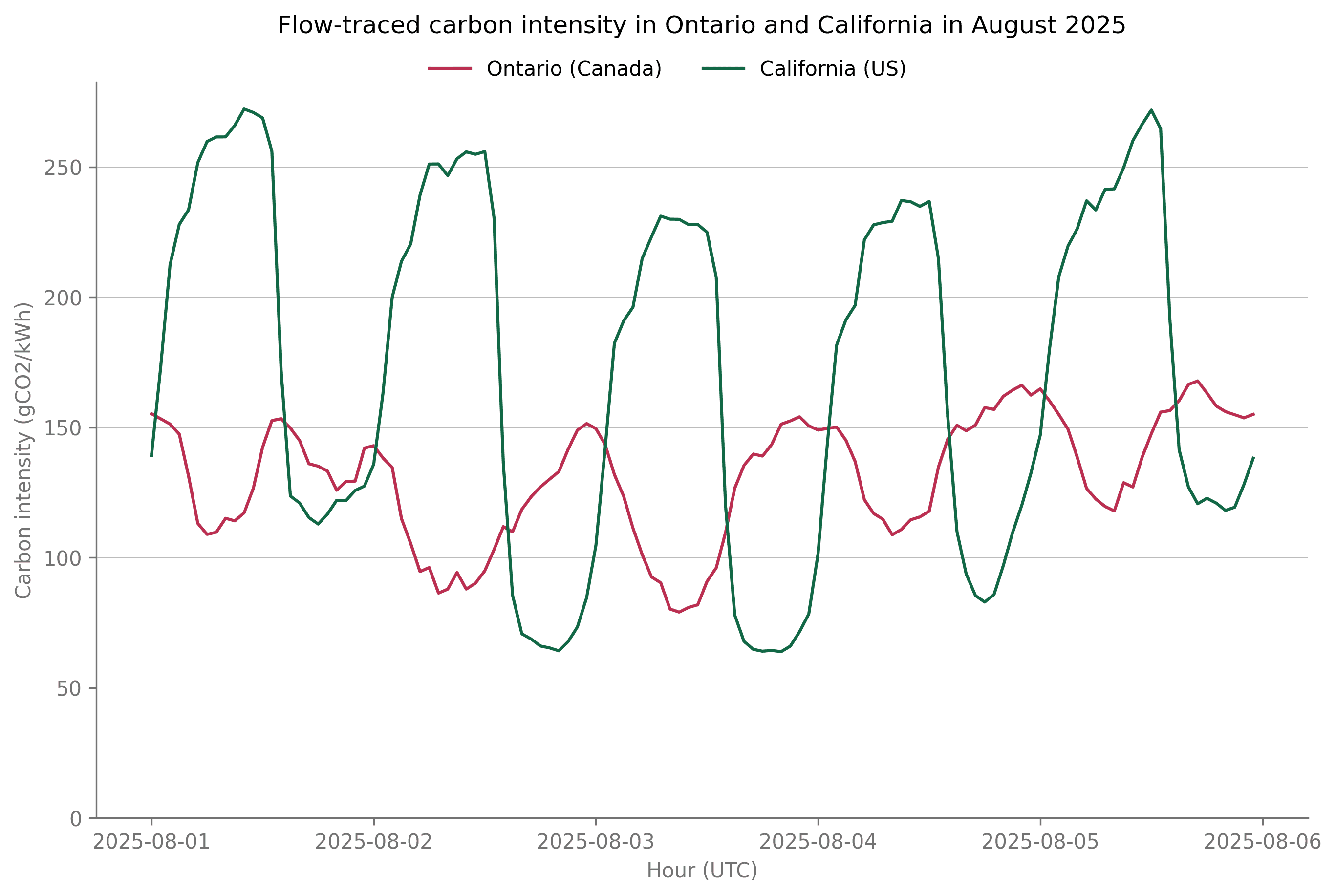
(Graph plotting Ontario and California's carbon intensity. Note how the curves are almost opposed in direction, leading to the fact that, depending on time of day, the location of lowest carbon intensity changes.)
It even depends on the week itself, as during some weeks, carbon intensity can remain higher in California even when solar generation is high. At the end of August, as wind generation was low and demand on the grid was high, the grid carbon intensity in California remained above the grid carbon intensity in Ontario for several consecutive days.
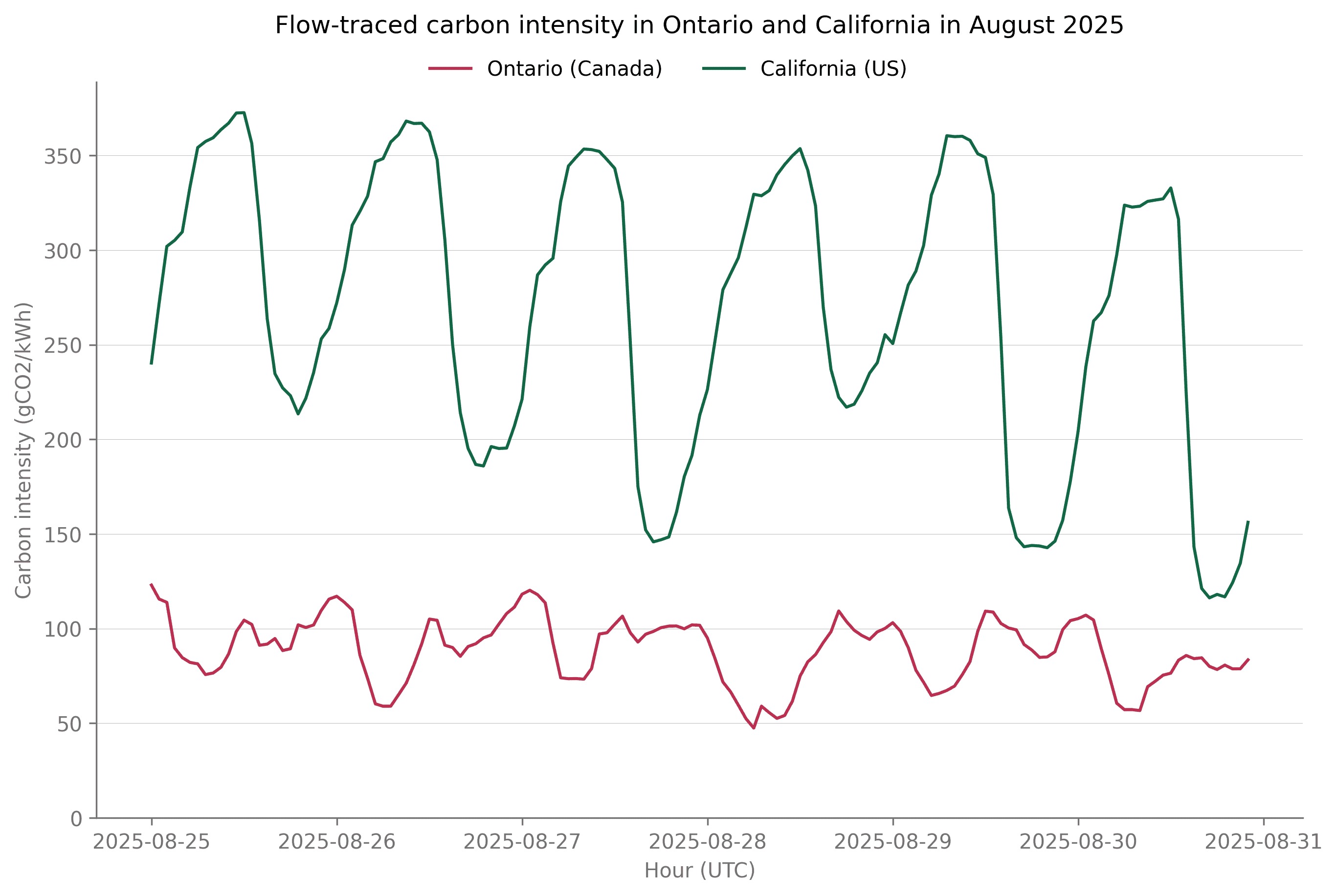
(A graph showing Ontario and California's carbon intensities, where Ontario's is significantly lower for the entire time)
We highlighted in previous lessons how historical data could already enable identifying best practices and recommendations to lower costs and emissions of IT. The above example shows the limitations of this approach, as a consequence of the very dynamic nature of the electricity grid.
Real-time data unlocks better decision-making and empowers your team and customers to more accurately identify the best locations to leverage cleaner and cheaper electricity. It enables live decisions that leverage spatial flexibility as best as possible. If we have a real-time view of the electricity grid, we can choose to run our workload on the grid with the lowest current carbon intensity.
What about the cost?
For a lot of companies, electricity represents a non-trivial portion of their costs. These companies tend to want to optimize for electricity costs (as well).
The difference in carbon intensity and electricity prices between grids, even located in the same region, can be very large at times. France and Germany have very different grid carbon intensities. But, at times, the price differences between the two grids can also get very large, as was the case several times in October this year.
In the example below, no matter which real-time signal you use to choose in optimising a workload (digital, or otherwise electricity-intense), you will opt for running it in France, with one exception: if you were to choose to run the workload at noon on the 3rd of October, and use the price signal as the optimisation parameters, you would choose Germany, with up to a 50% price discount when compared to France. You would also increase the carbon emissions of your workload by about 400%, demonstrating how some of the time, a lower price does not correlate with fewer emissions, which is important to keep in mind.
Note: Location-based flexibility with regard to price will depend on (1) your ability to move workloads. For IT jobs in distributed data centers, this is relatively easy, albeit locked on the cloud premises’ locations; and (2) on your price being both dynamic, and following the day-ahead price in a predictable way.
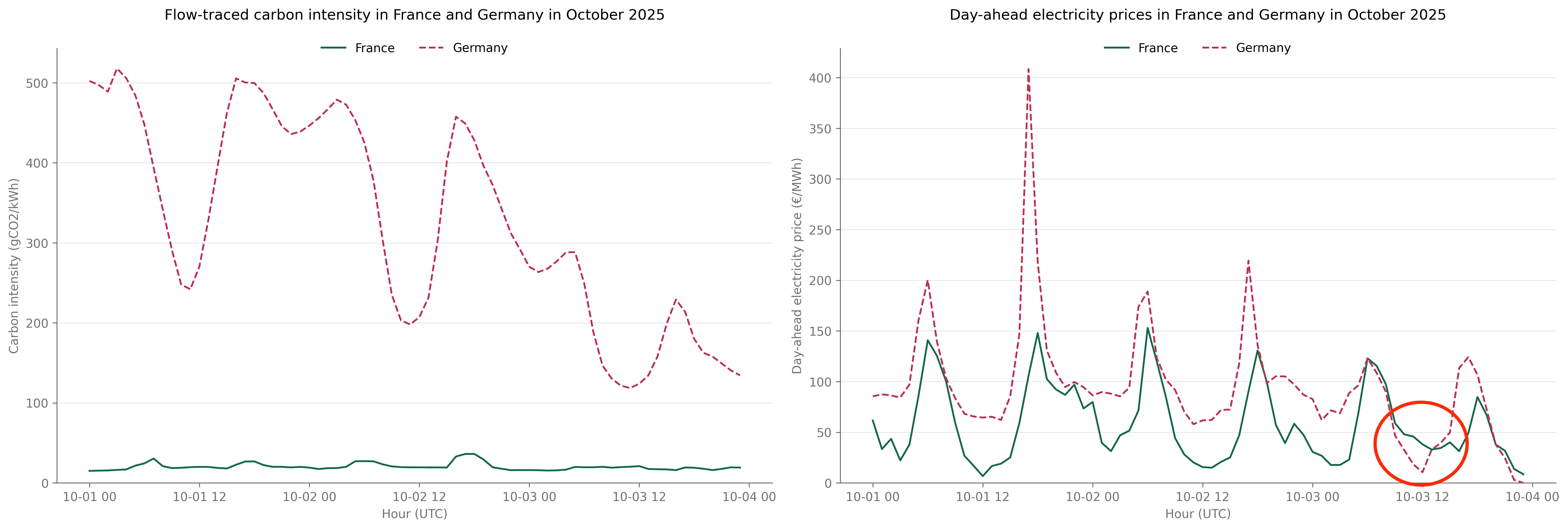
(Two graphs comparing the French and German grids in October 2025. For the entire duration, the carbon intensity is much lower in France. The price is also lower for almost the entire time. At some point, the price electricity of electricity in Germany drops below that of France, potentially saving 50% of the cost. The Carbon intensity, however, is about 4-5x in Germany, compared to France)
We highlighted how historical data could serve as a basis for decision-making, though with limitations, and how real-time data could alleviate some of these limitations when it comes to the location of the emissions.
Let’s now go to the next dimension relevant to flexibility:
Time flexibility
In the examples above, we talked about shifting loads based on the real-time view of electricity signals.
In reality, workloads do not run instantaneously. Big jobs, like for AI training, and even running database updates, machine learning algorithms, any sort of big data manipulation, will need to run for hours, sometimes days.
This introduces the problem of having to know how those signals will evolve into the future: If I can start a workload now, and it needs to run for the next 6 hours, what will the different signals look hour by hour, or even in 5-minute intervals?
What if we wanted to expand that timeline and instead of starting a job now, we wanted to schedule workloads into the future? This is where forecasting comes in. Forecasted data 72 hours into the future, on any signal, is available through Electricity Maps. Various providers offer different types of forecasts. At Electricity Maps, we’re forecasting all of our signals for the next 72 hours, in hourly and sub-hourly increments,
Our customers are using it for EV smart charging, scheduling updates, running cloud workloads at times of cheapest, or greenest electricity consumption.
Below, we’ll go through a couple of examples:
The benefits of forecast data
Let’s take a recent example to understand the benefits of forecast data. In the first week of October 2025, Storm Amy hit Europe, and thanks to significant wind speeds, several European grids broke records of renewable energy generation. However, the very low wind speeds in the second week of October led to spikes in electricity carbon intensity as well as electricity prices. In such a situation, 72-hour forecasts of electricity prices and carbon intensity enable shifting IT loads to times of lower cost and emissions.
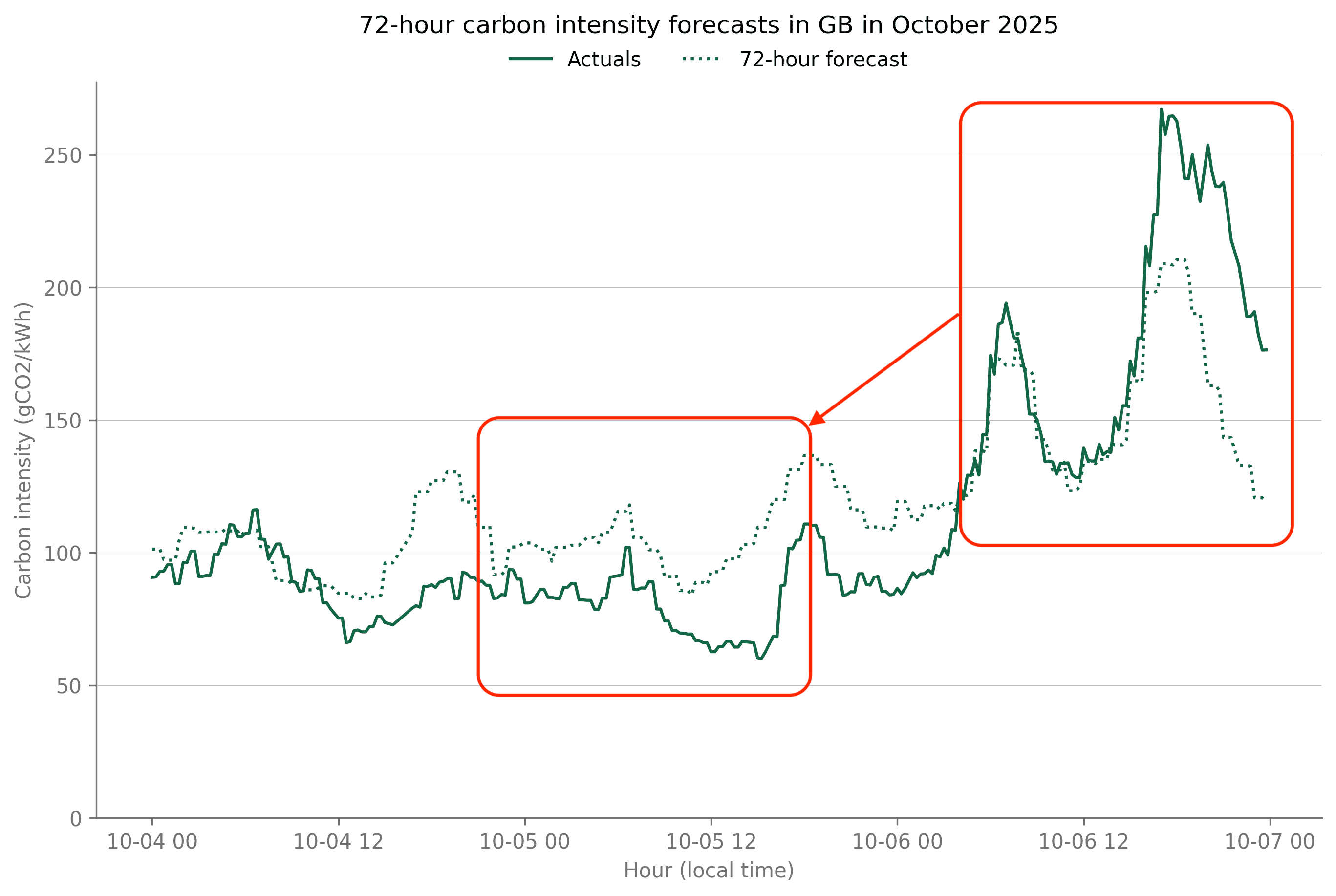
(Forecasted and Actuals carbon intensity forecasts in GB, October 2025. There is a big increase towards the end of the window, and we could save costs by shifting the workload to an earlier time)
With Electricity Maps forecasts, the spikes in carbon intensity on the 6th of October could have been predicted three days in advance, and as a consequence, flexible loads could have been shifted to different days, or at least to a different time of the day. Shifting workloads could have cut emissions by half in this example. The ability to shift loads between hours or days would obviously depend on the specific requirements of each workload and what flexibility each has, both in time and space, which leads us to the benefits of automation.
The benefits of automations
Automated load-shifting removes the constraint of individuals having to make decisions whether on historical, real-time, or forecasted data, and depending on the constraints each workload has. It’s what enables a seamless integration of load shifting into your workflows that, at the same time, maximizes emissions and cost reduction potentials while minimizing the impact on your team’s and clients’ work.
Each workload will likely have a set of constraints regarding where and when it should run, as well as characteristics such as its duration. The goal is to seamlessly optimize the scheduling of each workload to achieve a desired outcome. This outcome could, for example, be to minimize the electricity cost (by running at times of low day-ahead price), to minimize the electricity emissions (by running at times of low carbon intensity), or to help grid balancing (by running at times of low net load). This can be implemented with the help of the carbon-aware SDK from GSF or with the carbon-aware optimizer from Electricity Maps API (1), where users can choose duration, start and end times, available locations, and optimization metric to obtain the optimal time and location where to run the workload.

(Electricity Maps' Carbon Aware Optimizer end point, along with a sample request and response)
The untapped potential of load-shifting
The potential of load-shifting to reduce IT emissions and costs is huge! As an estimate of what savings can be achieved with load-shifting in time, we present below the average emissions and cost reduction of shifting flexible loads over a period of 24 hours in several grids worldwide.
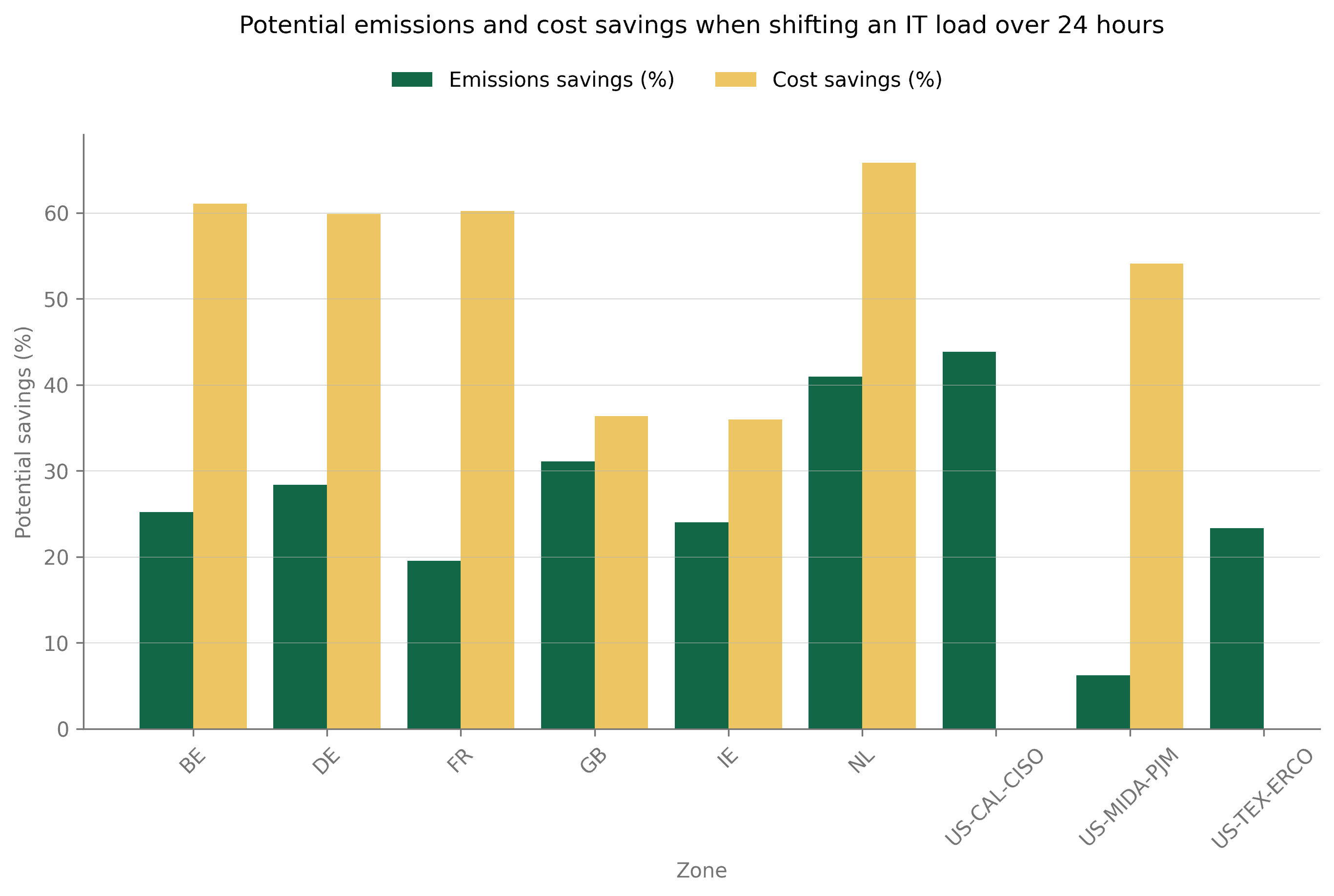
The potential savings were computed by calculating the average emissions and cost reductions of moving workloads over a 24-hour window for each hour of 2024. Price data was not available for US-CAL-CISO and US-TEX-ERCO. Moving workloads across a 24-hour window usually reduces their emissions by 30% and their cost by 50%.
Not all loads are flexible in time and can be shifted to different hours. But shifting those that can be will significantly reduce your IT cost and carbon footprint. IT workloads are also more inclined to be flexible in space rather than time. And here benefits can be huge as well. Carbon intensity and electricity prices can easily vary by a factor of 10 in neighboring countries or grids.
Set the best practices with automated load-shifting
Companies and working groups at the forefront of sustainability in IT are already going beyond the first steps of a Sustainable IT Monitoring journey. They are implementing space and time load shifting to leverage the full potential of emissions and cost reductions.
A few examples from our customers:
Google is running load shifting of their data centers based on Electricity Maps forecasts of the carbon intensity for the next 48 hours (2).
The Green Software Foundation released a carbon-aware SDK (3) that enables creating carbon-aware applications based on Electricity Maps forecasts. Microsoft leveraged the SDK to develop time and space load-shifting solutions for Vestas (4).
Monta offers a Smart Charging feature to hundreds of thousands of EVs (5).
What you will learn in next week’s lesson
This week marks the last deep dive into the steps of the Sustainable IT Journey. The sixth and last lesson, next week, will provide a summary of all the things we learnt throughout this course, as well as key takeaways.
Please submit any feedback you have about the course to help us improve. Also, take it as an occasion to submit any questions you may have on any topic we covered in this course since the first week, and we will answer them as part of the last lesson next week: 1-min survey