1. Introduction: Sustainable IT Monitoring & Grid Signals
The rising electricity consumption of the IT sector and the associated emissions mean sustainable IT is no longer a “nice-to-have” or a side project of developer teams. It becomes an operational necessity for all companies managing a large IT infrastructure and a growing customer demand for IT or Cloud service providers.
In 2024, data centers accounted for 1.5% of global electricity consumption (crypto excluded). Data transmission networks accounted for roughly the same share. Combined, this amounts to one-fifth of the US electricity generation in 2024. It shows that the significant contribution of IT to global electricity demand today does not only come from data centers, but extends to all IT infrastructure and services.
This electricity demand is significantly increasing. In the US, the expansion of data centres has been one of the main drivers of electricity demand growth over the last year and is projected to account for half of electricity demand growth between now and 2030. Data centers could account for one-third of the electricity demand in Ireland next year. As the electricity demand of data centers is set to double by 2030, it will exceed heavy industries' electricity consumption in some parts of the world.
This surge in power demand and the associated emissions are not limited to data centers but extend to all IT infrastructure and services. It raises multiple challenges, especially for grid connection, and calls for more IT infrastructure management.
This urges companies to more closely monitor IT emissions at a time when regulations are strengthening. It also requires more transparency from cloud and IT services providers, who must develop energy and emissions monitoring features or run the risk of losing customers and prospects to competition.
FinOps and GreenOps are known for being complementary, making operations more efficient and sustainable, reducing at the same time operating costs and emissions. With a more granular monitoring of IT electricity consumption and emissions, your company and your clients leverage both financial and sustainability benefits.
Emissions from IT are coming under more and more scrutiny today, as highlighted by the recent release of AI’s emissions reports and the discussions they sparked. Accurate monitoring of IT emissions becomes crucial, and leading companies as Cisco and Logic Monitor are paving the way by leveraging Electricity Maps data. Learn more in this course about how to develop Sustainable IT Monitoring features for your company and customers.
Course Objectives & Outline
This course addresses a major cornerstone when developing features of IT energy and emissions monitoring: gathering the right electricity grid data. It is relevant for all IT practitioners who develop - or want to develop - energy and emissions features for internal monitoring or B2B products.
By the end of this course, you will know:
What IT sustainability monitoring means and why this is a must-have for your company and your customers’ IT infrastructure management
What electricity grid data is, and what role it plays in the context of IT sustainability monitoring
Where to source this data from and how to select the right one for your use case
What a Sustainable IT Monitoring journey looks like
What a successful implementation looks like
The opportunities Sustainable IT Monitoring opens up for you and your customers, beyond emissions measurement and management
In Today’s lesson
In the rest of our introductory lesson today, we will cover the following:
Some basics of electricity grids’ dispatch, and what this means for electricity consumers
What electricity grids' signals are and why they are crucial in Sustainable IT Monitoring
Vocabulary
Electricity grid: Complex physical networks that connect electricity producers (traditional power plants, renewable producers, etc) and consumers (industries, households, etc), to enable electricity delivery.
Grid signal: A type of data that provides information about the state of the grid.
Electricity mix: A breakdown of the available electricity on the grid by technology of origin (wind, coal, etc). We distinguish between the production mix that only takes into account local generation and the flow-traced mix that takes into account electricity flows.
Electricity flows: Electricity (physically) transmitted between two areas. This can be either between or within an electricity grid.
Carbon-free and renewable energy percentages: Percentage of carbon-free and renewable sources in the origin of the electricity mix.
Electricity load: Total amount of electricity available (that can be consumed) on a power grid. It can also be referred to as demand.
Net load: The gap between electricity load and wind and solar generation (or generation by intermittent sources).
Carbon intensity: Emissions related to consuming electricity from the grid, expressed in gCO2/kWh.
Electricity prices: Price of electricity. This can either be market prices (corresponding to the price on wholesale markets) or retail prices (paid by end consumers). Several market prices exist, but the most common is the day-ahead market price
Electricity grids
Electricity grids are complex systems that connect electricity consumers and producers. Grid operators are responsible for ensuring demand equals generation at every second of the year, leveraging available production sources.
Because electricity demand and available production sources keep changing (for example, wind and solar generation), a multitude of parameters are fluctuating every second on the electricity grid.
As an image is worth a thousand words, here are two gifs that help better understand how things change over time and space on an electricity grid (here, the carbon intensity of electricity, which represents emissions from electricity consumption).
The first gif illustrates how carbon intensity fluctuates in time, between quarters, months, days, and hours on the Dutch grid.
The second gif illustrates how carbon intensity fluctuates in space for the same hour, depending on geographic granularity - here, the view switches from the grid level to the national level in the US and Canadian grids.

Carbon intensity fluctuates in time, between quarters, months, days, and hours on the Dutch grid.
Carbon intensity fluctuates in space for the same hour, depending on geographic granularity
Grid signals
There are a multitude of signals that can be followed about the grid. Some The fundamental ones are:
Load
Electricity mix per technology in MW
Electricity prices in €/MWh
But signals derived from the above can provide additional insights, such as:
Percentage of renewables or low-carbon sources on the grid
Carbon intensity of electricity in gCO2/kWh
Net load
The generation mix is very different from one grid to another (nuclear or not, penetration of renewables, phasing out of fossil fuels, …) as well as load profiles (electrification of heating and cooling, number of electric vehicles, presence of battery storage, behind-the-meter generation, …). This means fluctuations in space, between grids.
Fluctuations also happen in time, following renewable energy generation, times of peak consumption, seasonality in heating and cooling demand, time of the week, and time of the day, etc.
All signals fluctuate in space and time.
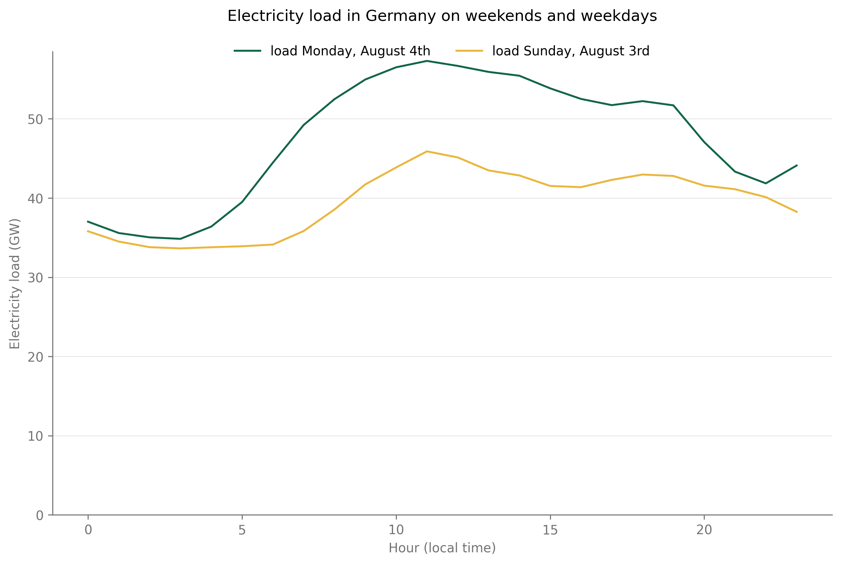
As a first example, let’s look at electricity load fluctuations within a day. Figures 1 and 2 illustrate how they differ in space (between Germany and PJM in the US), but also in time, between a weekday and a weekend, on the same grid (a Sunday and a Monday on the German grid).

Same day load fluctuations in Germany, compared to PJM (US)
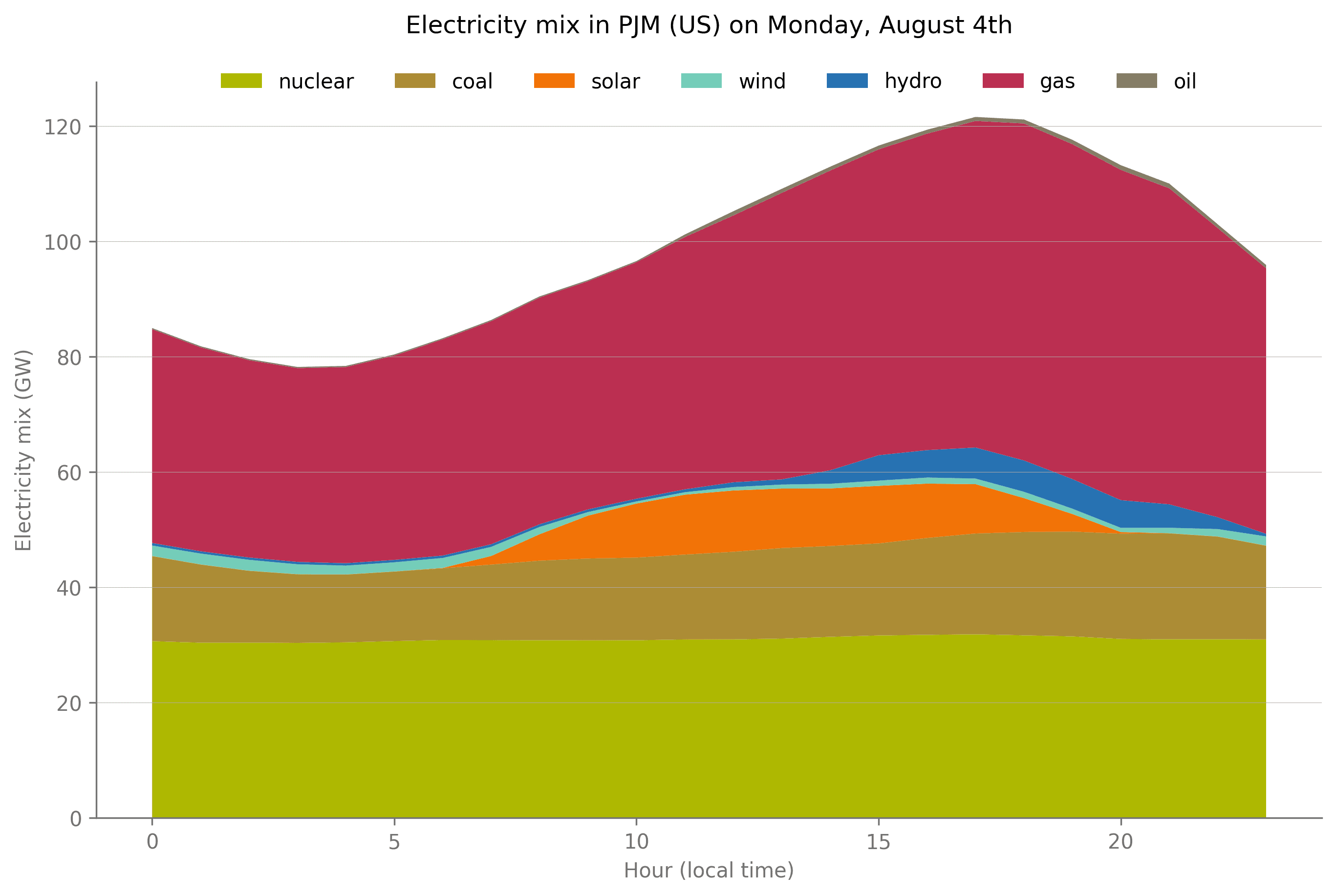
These fluctuations are also visible on the electricity mix side. The resources available to the grid operator to meet electricity demand fluctuate between hours but are also very different from one grid to another (between Germany and PJM in the US).
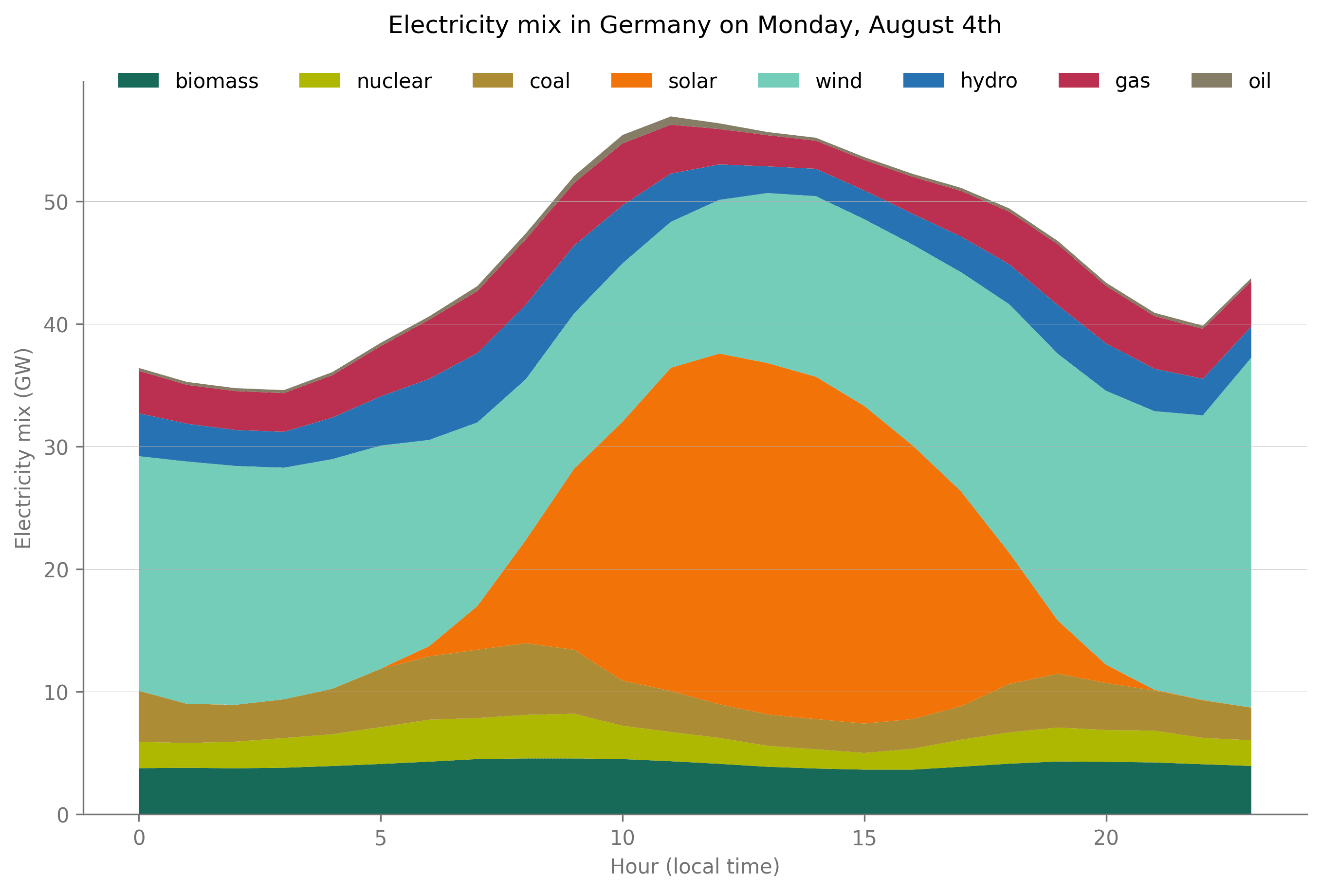
Electricity Mix in Germany on the 4th of August, 2025
You can explore how electricity demand and electricity mix fluctuate in space and time, and how these affect other characteristics of the grid such as the carbon intensity, or the share of renewables on our two freely available tools below:
Live map
Data explorer
This already highlights one key consideration when choosing the right data to ingest into your products and solutions: granularity matters! The granularity you need for your solution also depends on other factors, such as: how granular is your electricity consumption data? How frequent and granular can your monitoring be?
Insights increase with granularity. Moving from a yearly to an hourly granularity improves accuracy by 20% on average worldwide, and by more than 40% in several grids. Value is already achieved with small improvements in granularity; switching from a yearly to a monthly view already improves accuracy by more than 10% worldwide.
Learn more about how to source these grid signals and the key considerations to keep in mind for a successful data ingestion in the second lesson of this course.
The types of insights unlocked are not only a function of the granularity, but also of the time perspective considered:
Historical data enables trend analysis between years, accurate carbon accounting of IT emissions, dashboards of monthly activity with electricity consumption, and associated emissions.
Real-time data unlocks live insights on electricity carbon intensity and price, raises awareness among teams, and paves the way for optimization in time and space.
Forecasted data represents the cutting edge. Predictions over multiple days empower advanced and automated decision-making to optimize usage, increase efficiency, reduce costs, and emissions.
Going further
Let’s illustrate the importance of granularity when sourcing grid signals. We take as an example a data center located in Germany for which we approximate the load profile by the curve below:

Grid carbon intensity (hourly & monthly), and an example of a data center load curve in Germany
We consider two possible scenarios for the data center operator for monitoring their emissions: using a monthly carbon intensity of the German grid (282 gCO2/kWh in August), or using the hourly carbon intensity of the grid on the 4th of August 2025, already used in the example above.
To calculate the data center’s emissions from electricity consumption, the operator must multiply the load for each hour by the monthly emission factor (the same factor for each hour) or the hourly emission factor for each hour. With a monthly emission factor, the emissions computed per hour have the same profile as the load. Hours of high load are considered hours of high emissions, and inversely, overlooking how clean the grid might be at each hour, and how that fluctuates over time.
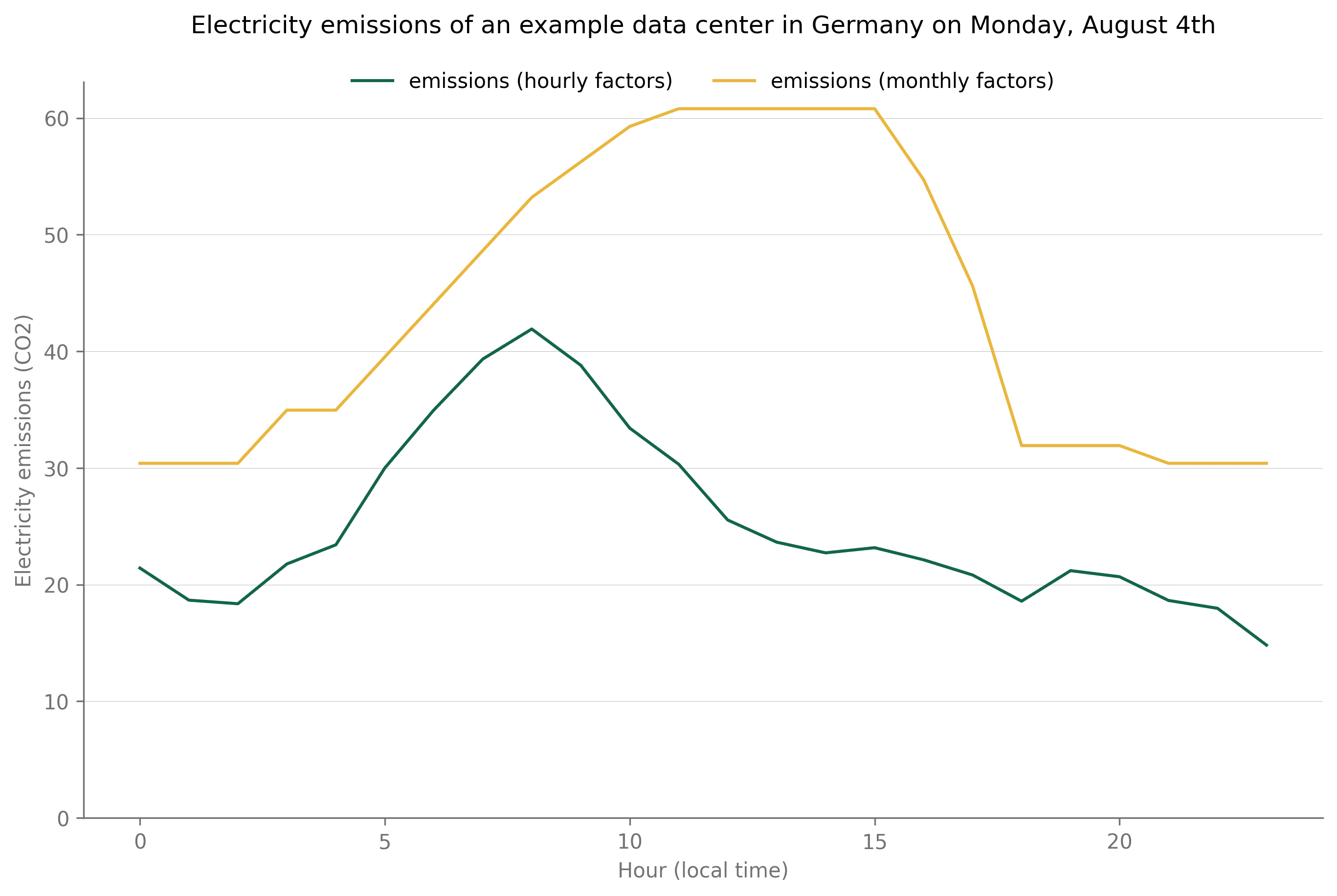
With hourly emissions factors, however, more insights are uncovered: the highest emissions are calculated at 8 am, even though the load is not at its peak yet, and inversely, emissions remain low at 2 pm, even though the data center remains at its peak consumption. The reason behind this is that the grid carbon intensity reached a peak at 8 am in the morning when consumption was high on the grid, and reached a minimum at the beginning of the afternoon when solar generation was high.
This example illustrates the importance of more granular signals in Sustainable IT Monitoring.
All numbers are available in the table below, where low values are highlighted in green and high values in red.

Table showing the data from the above graphs, with low values highlighted in green, and high values in red; The last two columns represent the difference in emissions values using monthly and hourly factors.
In closing
Sustainable IT Monitoring is no longer optional. With IT infrastructure consuming a rapidly growing share of global electricity, companies must monitor and manage their emissions.
This lesson introduced the fundamental concept that electricity grid signals fluctuate constantly across time and space, making granularity essential for accurate measurement. More granular data unlocks deeper insights, improves accuracy, and enables better decision-making for reducing both costs and emissions.
Next week's lesson will be a deep dive on grid signals. We'll be going into a lot more details for all of the above.
Check your inbox in a week!
We've left some references below 👇 And if you found this useful (or not, but read it anyway), please spare a minute to help us improve the course going forward: 1-min survey
References
1. Executive summary - Energy and AI - Analysis - IEA
2. Data centers & networks - IEA
3. United States of America - U.S. | Electricity Maps
4. Electricity Mid-Year Update 2025
5. Executive summary - Energy and AI - Analysis - IEA
6. Electricity 2024 - Analysis and forecast to 2026
7. Boon or bane: What will data centers do to the grid? | Canary media
8. Measuring the environmental impact of AI inference | Google Cloud Blog
9. Manage data center energy consumption with smart solutions - Cisco blogs
10. Webinar: Supporting Sustainability Reporting Requirements for your Managed Service Clients | LogicMonitor
11. Germany | App | Electricity Maps